Sensitivity Analysis
This page walks through the central API of SymbolicUncertainties.jl for the GUM §5.1 use case: closed-form propagation of measurement uncertainty through a user-supplied Julia function via symbolic sensitivity coefficients. The same machinery powers the elementary-function overloads, the apply escape hatch, the multi-variable propagate, and the vector-valued propagate_vector.
The relevant normative sections of JCGM 100:2008 are §5.1.2 (equation 10 — uncorrelated propagation), §5.1.3 (equation 11a/b — sensitivity coefficients cᵢ ≡ ∂f/∂xᵢ and individual contributions uᵢ(y) = |cᵢ|·u(xᵢ)), and §5.2.2 (equation 13 — correlated propagation with cross-covariance terms). For vector-valued measurands, JCGM 102:2011 (GUM Supplement 2) is the governing document.
Elementary functions on a single measurement
Sixteen Base mathematical functions accept a single SymbolicMeasurement and return a propagated measurement:
using Symbolics
using SymbolicUncertainties

@variables x σx
m = x ± σx

sin(m)        # u(sin(x)) = |cos(x)| · σx
cos(m)        # u(cos(x)) = |sin(x)| · σx
exp(m)        # u(exp(x)) = exp(x) · σx
log(m)        # u(log(x)) = σx / |x|
sqrt(m)       # u(√x)     = σx / (2·√x)
inv(m)        # u(1/x)    = σx / x²
The full list is sin, cos, tan, asin, acos, atan, sinh, cosh, tanh, exp, log, log2, log10, sqrt, abs, inv. Each propagates uncertainty via the standard sensitivity-coefficient formula u(f(x)) = |∂f/∂x| · u(x) from JCGM 100:2008 §5.1.2 (single-input specialisation).
Phase — the two-argument atan
atan(y, x) propagates the quadrant-preserving phase, with
\[\frac{\partial \varphi}{\partial y} = \frac{x}{x^2 + y^2}, \qquad \frac{\partial \varphi}{\partial x} = \frac{-y}{x^2 + y^2}.\]
This is the form a phase measurement takes in practice — a lock-in amplifier or a vector analyser reports quadrature components, and atan(y/x) throws away the quadrant that atan(y, x) keeps:
using Symbolics, SymbolicUncertainties, Logging
@variables Q σQ I σI

φ = with_logger(NullLogger()) do   # the origin cannot be excluded here
    atan(Q ± σQ, I ± σI)
end
φ.err
\[ \begin{equation} \sqrt{\mathtt{{\sigma}I}^{2} ~ \left( \frac{ - Q}{I^{2} + Q^{2}} \right)^{2} + \mathtt{{\sigma}Q}^{2} ~ \left( \frac{I}{I^{2} + Q^{2}} \right)^{2}} \end{equation} \]
At the origin the phase is undefined and both sensitivities diverge. The package warns rather than refuses, exactly as for a division whose denominator cannot be proven nonzero (REQ-140): the quantity is valid wherever the model is, and substitution decides.
Piecewise models are refused, and why
max, min and clamp raise an ArgumentError rather than propagating. This is a decision, not an omission. The GUM linearises the model around the input estimates (§5.1.2), and a piecewise model has no derivative at its switch point — so a first-order combined uncertainty is undefined exactly where the model does something interesting, and arbitrarily poor in a neighbourhood of it even where the derivative exists. A Monte Carlo method (JCGM 101:2008) is the right tool; the error message says so.
When the symbolic differentiation engine cannot find a closed-form derivative (e.g. for an iterative numerical solver wrapped as a Julia function, or for an unknown special function), the call raises an ArgumentError directing you at the apply escape hatch described below.
propagate — the central multi-variable API
propagate(f, [m₁, m₂, …, mₙ]) evaluates the user function f symbolically on the input estimates [m.val for m in ms], computes all sensitivity coefficients cᵢ = ∂f/∂xᵢ via Symbolics.derivative, and returns a new SymbolicMeasurement with the combined standard uncertainty per JCGM 100:2008 §5.1.2:
\[u_c²(y) = \sum_{i=1}^{N} \left(\frac{\partial f}{\partial x_i}\right)^2 u^2(x_i)\]
A two-input addition:
using Symbolics
using SymbolicUncertainties

@variables a σa b σb
a_m = a ± σa
b_m = b ± σb

result = propagate((x, y) -> x + y, [a_m, b_m])
# val: a + b
# err: sqrt(σa² + σb²)
A nonlinear three-input combination follows the same shape — every sensitivity coefficient is computed automatically:
using Symbolics
using SymbolicUncertainties

@variables a σa b σb c σc
result = propagate(
    (x, y, z) -> x * y * z,
    [a ± σa, b ± σb, c ± σc],
)
# err: sqrt((b·c·σa)² + (a·c·σb)² + (a·b·σc)²)
Worked example — voltage divider
The textbook voltage divider Vout = Vin · R₂ / (R₁ + R₂) is a three-input non-linear measurand. With distinct symbolic inputs:
using Symbolics
using SymbolicUncertainties

@variables Vin σVin R1 σR1 R2 σR2

Vin_m = Vin ± σVin
R1_m  = R1 ± σR1
R2_m  = R2 ± σR2

Vout = propagate(
    (Vin, R1, R2) -> Vin * R2 / (R1 + R2),
    [Vin_m, R1_m, R2_m],
)
The sensitivity coefficients are:
\[\frac{\partial V_{out}}{\partial V_{in}} = \frac{R_2}{R_1 + R_2} \qquad \frac{\partial V_{out}}{\partial R_1} = -\frac{V_{in} R_2}{(R_1 + R_2)^2} \qquad \frac{\partial V_{out}}{\partial R_2} = \frac{V_{in} R_1}{(R_1 + R_2)^2}\]
and the propagated uncertainty is
\[u(V_{out}) = \sqrt{ \left(\frac{R_2}{R_1+R_2}\right)^2 \sigma_{V_{in}}^2 + \left(\frac{V_{in}\,R_2}{(R_1+R_2)^2}\right)^2 \sigma_{R_1}^2 + \left(\frac{V_{in}\,R_1}{(R_1+R_2)^2}\right)^2 \sigma_{R_2}^2 }\]
Vout.err matches this expression up to symbolic simplification and is asserted exactly by test/examples/test_voltage_divider.jl.
The voltage divider is not one of the worked examples in JCGM 100:2008 Annex H (which lists end-gauge calibration in H.1, simultaneous resistance-and-reactance measurement in H.2, thermometer calibration in H.3, etc.). It is retained here as a standard textbook illustration of the product / quotient rule.
Figure — a sensitivity coefficient is a function, not a constant
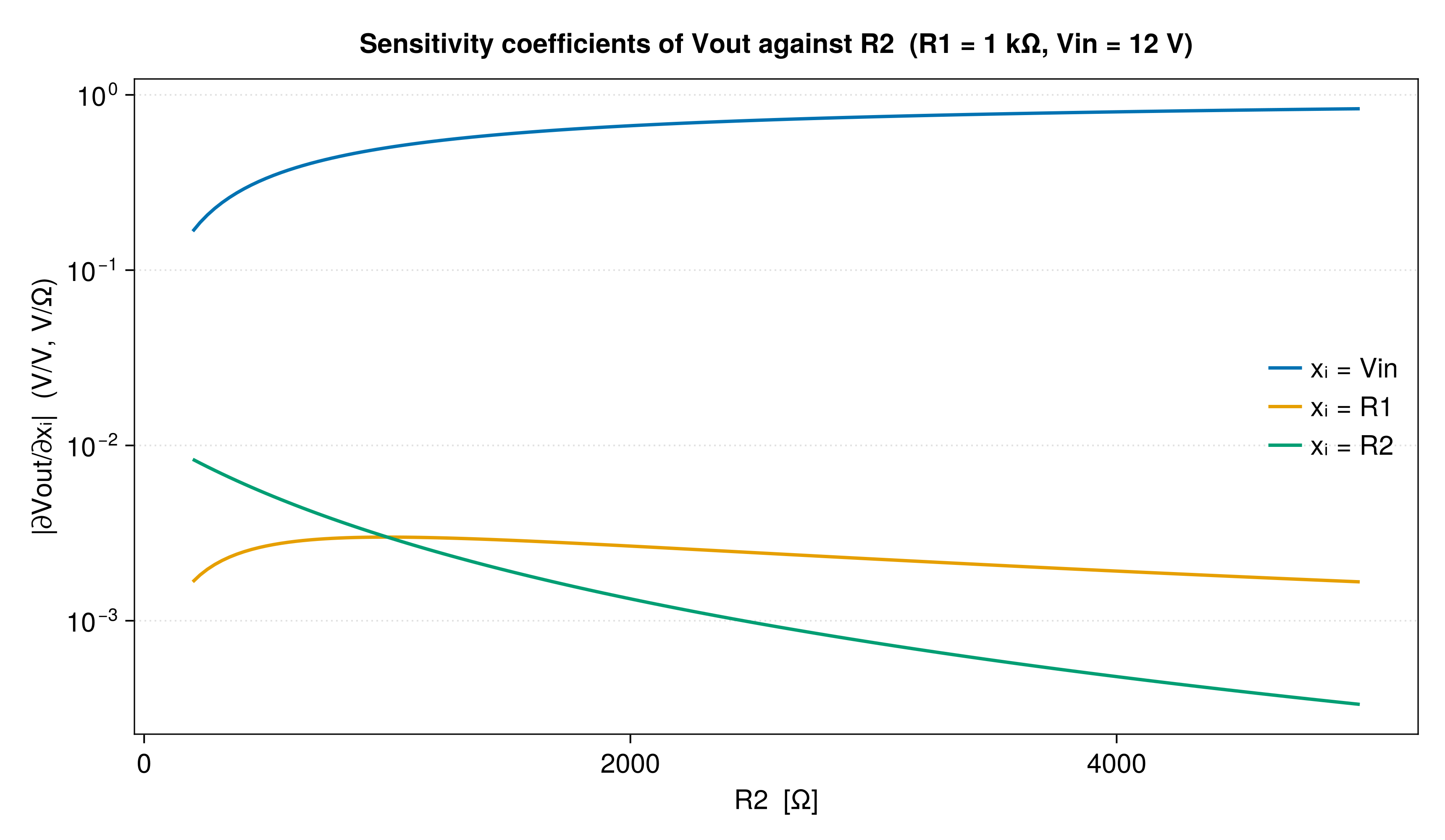
sensitivity_coefficient for each input of the same divider, evaluated over a sweep of R2. The two resistor curves cross near R2 = R1: below it the output is more sensitive to R2, above it to R1. A coefficient is a function of the operating point, so a budget computed at one R2 does not carry over to another.
The three curves do not share a unit — ∂Vout/∂Vin is dimensionless while ∂Vout/∂R is V/Ω — so their heights are not comparable with one another. What is comparable is each one's contribution, coefficient times standard uncertainty, which is what the Uncertainty Budget page plots.
Generated by docs/figures/make_figures.jl from the fixtures in docs/figures/fixtures.jl: computed by the package itself, never copied from a standard (REQ-307, REQ-312).
Identity cancellation
An expression that reuses the same measurement cancels exactly, through the plain operators:
julia> m = 8.4 ± 0.7
8.4 ± 0.7

julia> m - m
0.0 ± 0

julia> m / m
1 ± 0

julia> m + m
16.8 ± 1.4
Identity lives in the type, and propagate produces the same answers as the operators because it is a convenience over them rather than a separate path:
using Symbolics
using SymbolicUncertainties

@variables x σx
m = x ± σx

propagate(y -> y - y,         [m])    # → 0 ± 0
propagate(y -> y / y,         [m])    # → 1 ± 0
propagate(y -> y*y*y - y^3,   [m])    # → 0 ± 0
The plain binary operators do this too — there is no right and wrong way to write the same model:
m - m        # → 0 ± 0
m / m        # → 1 ± 0
m + m        # → 2x ± 2σx, not σ√2
propagate remains available for models expressed as a function of several inputs, but it is now a convenience over those operators rather than a separate, more correct path. The regression tests are test/examples/test_identity_cancellation.jl and test/chainrule/test_operand_identity.jl.
See Uncertainty Sources for the representation that makes this work.
apply — the escape hatch
When the symbolic differentiation engine cannot find a closed-form derivative for the user's function f, calling f(m) directly or propagate(f, [m]) raises ArgumentError whose message names the function and points at apply:
using Symbolics
using SymbolicUncertainties

# Declare a function whose derivative Symbolics cannot find.
@register_symbolic my_special_function(x)

@variables x σx
m = x ± σx

# Calling propagate (or the function directly) on a measurement
# raises ArgumentError because Symbolics has no derivative rule.
# The error message tells you to use `apply`.

# Supply the derivative explicitly as a symbolic expression in m.val:
my_df = 2 * x   # whatever the closed-form derivative is
result = apply(my_special_function, m; derivative = my_df)
# val: my_special_function(x)
# err: |2x| · σx
The derivative keyword takes a symbolic expression in the same variable as m.val, not a Julia function. To use a function-style derivative, evaluate it at m.val first:
df_fn(x) = 2 * x
apply(my_special_function, m; derivative = df_fn(m.val))
When called without the derivative keyword, apply(f, m) delegates to propagate(f, [m]) and uses Symbolics.derivative in the normal way. This makes apply a strict generalisation of propagate(f, [m]) that adds the explicit-derivative override.
Correlated inputs — propagate(f, ms, Σ)
When the input quantities are correlated, supply a covariance matrix Σ as the third argument. The library applies the correlated form of the law of propagation, JCGM 100:2008 §5.2.2 equation (13), including all cross-covariance terms:
\[u_c²(y) = \sum_{i,j} \frac{\partial f}{\partial x_i} \frac{\partial f}{\partial x_j} \, u(x_i, x_j)\]
using Symbolics
using SymbolicUncertainties

@variables x σx y σy ρ

x_m = x ± σx
y_m = y ± σy

# Symbolic 2×2 covariance matrix with correlation coefficient ρ.
Σ = [σx^2  ρ*σx*σy
     ρ*σx*σy  σy^2]

result = propagate((a, b) -> a + b, [x_m, y_m], Σ)
# val: x + y
# err: sqrt(σx² + σy² + 2·ρ·σx·σy)
Wrong-shape covariance matrices raise DimensionMismatch:
# 3×3 Σ with a 2-element measurement vector → DimensionMismatch
# 2×3 non-square Σ                          → DimensionMismatch
When Σ is diagonal (off-diagonal entries are zero), the correlated method produces results mathematically equivalent to the uncorrelated propagate(f, [m₁, m₂]). This is the FR-010 strict-generalisation invariant.
Vector-valued measurands — propagate_vector
For multi-output models, propagate_vector(f, ms) accepts a function f that returns a tuple or vector of derived quantities and returns a Vector{SymbolicMeasurement} whose .err fields come from the symbolic Jacobian:
using Symbolics
using SymbolicUncertainties

@variables r σr θ σθ
r_m = r ± σr
θ_m = θ ± σθ

# Polar-to-Cartesian conversion: 2 inputs, 2 outputs.
ms = propagate_vector(
    (r, θ) -> (r * cos(θ), r * sin(θ)),
    [r_m, θ_m],
)

# ms[1].val = r·cos(θ); ms[1].err = sqrt((cos(θ))²·σr² + (r·sin(θ))²·σθ²)
# ms[2].val = r·sin(θ); ms[2].err = sqrt((sin(θ))²·σr² + (r·cos(θ))²·σθ²)
Each output measurement carries only its marginal propagated uncertainty (the diagonal of J · Σ_in · J^T where J is the symbolic Jacobian and Σ_in is a diagonal matrix of input variances). The full output covariance matrix is not exposed here; users who need it can call Symbolics.jacobian(vals, xs) directly and assemble it themselves.
This implements the methodology of JCGM 102:2011 (GUM Supplement
- for multi-output measurands.
Optional CAS-grade simplification via Giac.jl
All propagated .err fields are routed through an internal hook, _simplify_for_report, which defaults to Symbolics.simplify. The Symbolics rewriter handles polynomial and rational forms well but leaves certain trigonometric or transcendental identities unreduced. For example, Symbolics.simplify(-tan(x) + sin(x)/cos(x)) returns (sin(x) - cos(x)·tan(x)) / cos(x) rather than 0.
Loading Giac.jl activates the SymbolicUncertaintiesGiacExt package extension, which overloads _simplify_for_report to route expressions through Giac's CAS. Whenever Giac fails or errors, the default Symbolics.simplify is used instead, so every pre-existing test continues to pass. Beyond reducing identities the default engine leaves alone, it also avoids three upstream defects that make Symbolics.simplify return a wrong answer or throw — see below.
using Symbolics
using Giac            # activates the extension
using SymbolicUncertainties

@variables x σx
m = x ± σx

# d/dx[tan(x) − sin(x)/cos(x)] ≡ 0, but the Symbolics default leaves
# the expression in an unreduced form.
result = propagate(y -> tan(y) - sin(y) / cos(y), [m])
result.err   # → 0   (with Giac loaded)
             # → an unsimplified expression (without Giac)
The extension uses the Giac.to_giac / Giac.to_symbolics round-trip together with Giac's simplify command. Load it whenever sensitivity expressions involve trigonometric, hyperbolic, or transcendental identities that the default engine leaves unreduced.
The fallback is defensive by design: a future Giac version change or an input expression Giac cannot parse cannot make the simplification step worse than the Symbolics baseline.
Upstream defects that Giac avoids
Giac is not only a stronger simplifier. Three defects in the default Symbolics.simplify path are reached by ordinary metrological input, and Giac returns the right answer on all three:
| upstream issue | Symbolics.simplify | via Giac |
|---|---|---|
| SymbolicUtils#1050 | 1e-9(3.0 + 5.0x)/sqrt(1 + x) → 5.0e-9sqrt(1 + x), a different function (15 % error) | both numerator terms kept, departure only 4.3e-15 relative |
| SymbolicUtils#1051 | OverflowError on Rational coefficients with a large denominator | completes, using arbitrary-precision integers |
| SymbolicUtils#1044 | BoundsError on (-U)^2 | U^2 |
The first defect is the one that matters most here: it returned exactly 0 for a non-zero sensitivity in the thermocouple model, which would have deleted an uncertainty source and understated u_c.
This package does not depend on Giac to be correct. Both failure modes are guarded internally — a simplified zero is re-checked numerically before any source is dropped, and simplification never propagates an exception. Those guards are backend-agnostic on purpose, and they are what makes the answer the same whether or not Giac is loaded. See Limitations for the reasoning.
What loading Giac buys you is that the expressions are also readable: without it, a sensitivity whose simplification is refused is reported in its unsimplified form.
using Symbolics, Giac

@variables x
e = 1e-9 * (3.0 + 5.0x) / sqrt(1 + x)

Symbolics.simplify(e)
# 5.0e-9sqrt(1 + x)                          ← wrong

Giac.to_symbolics(Giac.Commands.normal(Giac.to_giac(e)))
# (2.999999999999987e-9 + 4.999999999999979e-9x)*inv((1 + x)^(1//2))
Three caveats before treating Giac as a safety net:
- It is optional, and most installations will not have it. A correctness property that depends on an optional extension is not a correctness property, which is why the guards above exist.
- Its own failure is silent. Giac emits a parse error on some mangled identifiers and falls back to
Symbolics.simplify(upstream-bugs.mdUB-005) — that is, back onto the defects above, with only a@debugrecord to say so. - It is not exactly value-preserving. The round trip through Giac's decimal/rational representation moves float coefficients in the fifteenth digit, as the
2.999999999999987e-9above shows. Harmless numerically, but expressions will not compareisequalto their inputs.
API reference
SymbolicUncertainties.apply — Function
apply(f, m::SymbolicMeasurement; derivative = nothing) -> SymbolicMeasurementApply a single-argument function f to a measurement m, returning the propagated measurement.
When derivative === nothing (the default), apply delegates to propagate(f, [m]), which uses Symbolics.derivative to compute the sensitivity coefficient. This path produces results identical (after simplification) to calling f(m) directly for any function the symbolic engine can differentiate.
When derivative is a Symbolics.Num expression (in the same variable as m.val), apply uses it directly and computes u(f(x)) = |derivative| · u(x), skipping the symbolic differentiation step. This is the escape hatch for functions whose derivative the symbolic engine cannot find — propagate(f, [m]) would raise ArgumentError directing the user here.
The derivative keyword takes a symbolic expression, not a Julia function. To use a function-style derivative, evaluate it at m.val first:
my_df(x) = 2*x
apply(f, m; derivative = my_df(m.val))
Implements the methodology of JCGM 100:2008 §5.1.3 (sensitivity coefficients). Traces REQ-022.
SymbolicUncertainties.propagate — Function
propagate(f, ms::AbstractVector{SymbolicMeasurement}) -> SymbolicMeasurementPropagate uncertainty through a user-supplied Julia function f of length(ms) arguments, evaluated on the input measurements ms, implementing JCGM 100:2008 §5.1.2 equation (10) for uncorrelated inputs:
u_c²(y) = Σᵢ (∂f/∂xᵢ)² · u²(xᵢ)The sensitivity coefficients ∂f/∂xᵢ are obtained symbolically from Symbolics.derivative evaluated on f(m₁.val, m₂.val, …, mₙ.val). The result is a new SymbolicMeasurement whose val field is the symbolic output expression and whose err field is the propagated combined standard uncertainty (simplified once via Symbolics.simplify).
When the user function reuses the same input mᵢ multiple times in its body, symbolic differentiation correctly handles the cancellation. For example, propagate(x -> x - x, [m]) returns a measurement with zero uncertainty — as does m - m written directly, since M11 moved identity tracking into the type.
Raises ArgumentError (REQ-021 / FR-004) if the symbolic engine cannot compute a closed-form derivative for any input. Use the apply(f, m; derivative = ...) escape hatch in that case.
Edge cases:
length(ms) == 0returnsSymbolicMeasurement(Num(f()), Num(0))— empty sum has zero variance.freturning a value independent of anyms[i]returns zero propagated uncertainty.
Implements the methodology of JCGM 100:2008 §5.1.2 equation (10). Traces REQ-030, REQ-110.
SymbolicUncertainties.propagate_vector — Function
propagate_vector(f, ms::AbstractVector{SymbolicMeasurement}) -> Vector{SymbolicMeasurement}Propagate uncertainty through a multi-output function f of length(ms) arguments. f(ms[1].val, ..., ms[N].val) must return something collect-able (a Tuple, Vector, or any iterable producing M symbolic outputs).
Returns a Vector{SymbolicMeasurement} of length M, where each output measurement carries:
val— the symbolic output expressionerr— the marginal propagated standard uncertainty of that output, i.e. the diagonal ofJ · Σ_in · J^TwhereJis theM × Nsymbolic Jacobian andΣ_inis the diagonal matrix of input variancesu²(xₖ)
At M2 the inputs are assumed uncorrelated. The full cross-output covariance matrix J · Σ_in · J^T is not exposed by this method; users who need it can call Symbolics.jacobian(vals, xs) directly and combine it with Σ_in themselves.
Implements the methodology of JCGM 102:2011 (GUM Supplement 2). Traces REQ-033, REQ-110.
Base.atan — Method
Base.atan(y::SymbolicMeasurement, x::SymbolicMeasurement)Propagate the two-argument arctangent — the quadrant-preserving phase atan(y, x) — with sensitivity coefficients
∂φ/∂y = x / (x² + y²) ∂φ/∂x = -y / (x² + y²)This is the form a phase measurement actually takes: a lock-in amplifier or a vector analyser reports quadrature components, and atan(y/x) loses the quadrant that atan(y, x) keeps.
At the origin the phase is undefined and both sensitivities diverge. As with the REQ-140 division guard, the package warns rather than refuses when x² + y² cannot be proven nonzero at build time (upstream-bugs.md UB-003): the returned quantity is valid wherever the model is, and substitution decides.
Implements the methodology of JCGM 100:2008 §5.1.3. Traces REQ-023.
Base.log10 — Method
Base.log10(m::SymbolicMeasurement)Propagate the base-10 logarithm using ∂log10(x)/∂x = 1 / (ln(10) · x). Assumes x > 0. Implements JCGM 100:2008 §5.1.2. Traces REQ-020.
Base.abs — Method
Base.abs(m::SymbolicMeasurement)Propagate abs using ∂|x|/∂x = sign(x). The sensitivity coefficient is piecewise (+1 for x > 0, -1 for x < 0); since the propagation formula multiplies by |c|, the propagated standard uncertainty is simply m.err for any non-zero x. Implements JCGM 100:2008 §5.1.2. Traces REQ-020.