Linearity Check
The GUM §5.1.1 note reminds the user that the law of propagation of uncertainty is a first-order Taylor approximation valid when higher-order terms are negligible. check_linearity surfaces that assumption actively: it returns a per-variable dimensionless nonlinearity indicator
\[\eta_i = \frac{\partial^2 f / \partial x_i^2 \cdot \sigma_i^2} {2 \cdot \partial f / \partial x_i \cdot \sigma_i}\]
— the ratio of the neglected second-order Taylor term to the retained first-order term. |ηᵢ| ≪ 1 means the linear propagation is safe; |ηᵢ| > 0.1 signals a regime where Monte Carlo methods (JCGM 101:2008, MonteCarloMeasurements.jl) should be used instead.
The two signalling behaviours
Symbolic indicator
using Symbolics, SymbolicUncertainties

@variables x σx
η = check_linearity(a -> exp(a), [x ± σx])
# η[σx] is the symbolic expression for ηᵢ.
Dict{Symbolics.Num, Symbolics.Num} with 1 entry:
σx => σx / 2For any SymbolicMeasurement-producing function, the diagonal ∂²f/∂xᵢ² and the first derivative ∂f/∂xᵢ are computed via Symbolics.derivative, through the same guarded helper the elementary functions use. A per-input σᵢ key in the returned Dict{Num, Num} maps to the symbolic ηᵢ.
The argument of exp, like that of every transcendental function, must be dimensionless — exp(1 V) is not a quantity. The x below is therefore a genuinely dimensionless input, and annotating it with a unit would be a physical error rather than an improvement. The nonlinearity indicator η is dimensionless for the same reason: it compares a second-order term with a first-order one, and a ratio of two quantities of the same dimension has none.
Runtime threshold @warn
check_linearity(
    a -> exp(a),
    [x ± σx];
    values = Dict(x => 1.0, σx => 0.5),
)
# ┌ Warning: check_linearity: |η| = 0.25 exceeds the GUM
# │ §5.1.1 linearity threshold of 0.1 for variable `σx`.
# │ The first-order propagation formula may be inadequate
# │ — consider Monte Carlo methods
# │ (MonteCarloMeasurements.jl / JCGM 101:2008). (REQ-181)
# └
Dict{Symbolics.Num, Symbolics.Num} with 1 entry:
σx => σx / 2The values keyword triggers a numeric threshold check: for each ηᵢ that evaluates to a concrete Float64 exceeding 0.1, a runtime @warn fires per REQ-181. Entries with partial / un-substituted values are silently skipped (the indicator in the returned dict is still symbolic for manual inspection).
No warning at low nonlinearity
check_linearity(
    a -> exp(a),
    [x ± σx];
    values = Dict(x => 1.0, σx => 0.1),
)
# η = 0.05 — below threshold → no warning.
Dict{Symbolics.Num, Symbolics.Num} with 1 entry:
σx => σx / 2Worked example — linear vs nonlinear contrast
@variables x σx
η_lin = check_linearity(a -> 2a + 3, [x ± σx])
# η_lin[σx] simplifies to 0 — exact linearisation.

η_nl = check_linearity(a -> exp(a), [x ± σx])
# η_nl[σx] = σx / 2 — grows with σx.
Dict{Symbolics.Num, Symbolics.Num} with 1 entry:
σx => σx / 2This is the REQ-155 acceptance criterion.
Figure — the indicator against the input's relative uncertainty
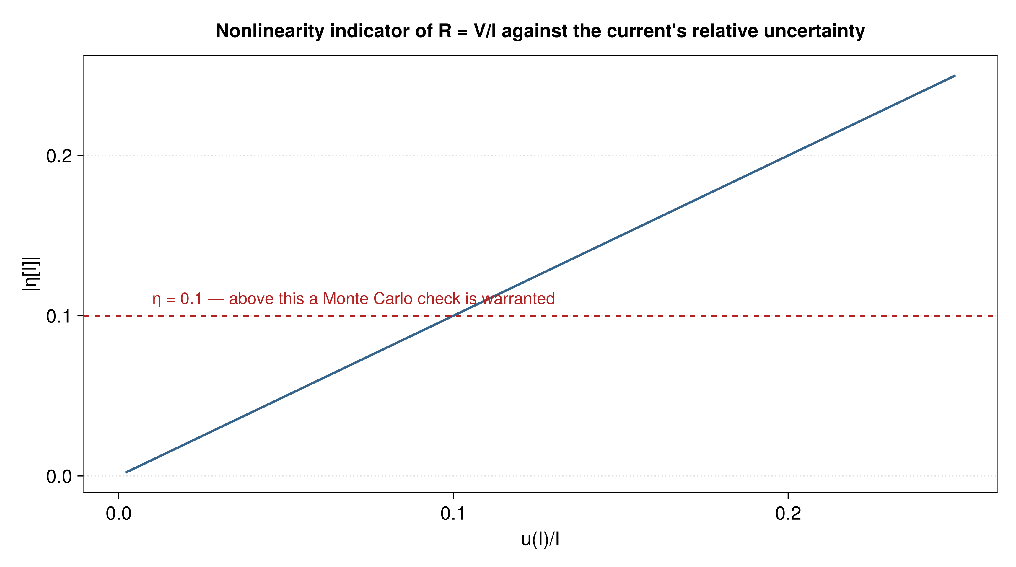
check_linearity evaluated for R = V/I while the current's relative uncertainty grows. For a quotient the indicator is the relative uncertainty itself — a straight line of slope one through the origin — so the §5.1.1 threshold of 0.1 is reached exactly at u(I)/I = 0.1. Left of that crossing the first-order formula is adequate; right of it this page sends you to Monte Carlo.
Generated by docs/figures/make_figures.jl from the fixtures in docs/figures/fixtures.jl: computed by the package itself, never copied from a standard (REQ-307, REQ-312).
No silent higher-order correction (REQ-182)
check_linearity is a pure observer: running it does not change any propagation output. Before-and-after comparisons of propagate(f, [m]) are bit-identical irrespective of whether check_linearity has been called.
y1 = propagate(a -> exp(a), [x ± σx])
check_linearity(a -> exp(a), [x ± σx])     # no side effect
y2 = propagate(a -> exp(a), [x ± σx])
# y1.val == y2.val and y1.err == y2.err symbolically.
\[e^{x} \pm \sqrt{\mathtt{{\sigma}x}^{2} ~ \left( e^{x} \right)^{2}}\]
Asserted by test/linearity/test_no_higher_order_correction.jl.
Scope — diagonal only
check_linearity tracks the diagonal second derivative ∂²f/∂xᵢ² only, not the mixed partials ∂²f/∂xᵢ∂xⱼ. For a measurand whose nonlinearity lives in the cross terms this indicator under-reports it — a product is the extreme case, since every ∂²(ab)/∂xᵢ² is zero while all of its nonlinearity sits in ∂²(ab)/∂a∂b.
linearisation_bound includes the mixed partials and returns a rigorous bound rather than an indicator; use it when the diagonal is not enough.
Error paths
- Unresolved second derivative →
ArgumentErrornoting that there is noderivative_2override — no analogue of theapply(f, m; derivative = ...)escape hatch exists for second derivatives. - Empty input list → empty dict, no error, no
fcall.
Silencing the safety-warning chatter
The ηᵢ formula contains a division by 2·cᵢ·σᵢ, which is usually symbolic, so the REQ-140 @warn fires from within check_linearity. In tests and REPLs this is typically silenced via:
using Logging
Logging.with_logger(Logging.NullLogger()) do
    check_linearity(a -> exp(a), [x ± σx])
end
Dict{Symbolics.Num, Symbolics.Num} with 1 entry:
σx => σx / 2The test suite uses exactly this pattern.
API reference
From indicator to bound
check_linearity is a heuristic: it evaluates a second-derivative ratio at a point and warns past |η| > 0.1. It is also diagonal-only — it looks at ∂²f/∂xᵢ² and ignores the mixed partials. That gap is not academic:
using Symbolics
using SymbolicUncertainties
@variables a σa b σb

check_linearity(*, [a ± σa, b ± σb])   # η = 0 for both inputs
Dict{Symbolics.Num, Symbolics.Num} with 2 entries:
σb => 0
σa => 0A product's Hessian has a zero diagonal, so the indicator calls a·b linear. It is not: all of its nonlinearity sits in ∂²(ab)/∂a∂b = 1.
linearisation_bound answers the question the indicator only gestures at — by how much can the first-order result be wrong? — and answers it rigorously:
The true worst error over that region is 0.0582, so the bound contains it and stays tight:
linearisation_bound(exp, [a ± σa]; coverage_factor = 2,
values = Dict(a => 1.0, σa => 0.1))0.06640233845473095Taylor's theorem with the Lagrange remainder bounds the error by ½ Σᵢⱼ max|Hᵢⱼ| · (k·uᵢ)(k·uⱼ), with each Hᵢⱼ bounded by interval arithmetic over the coverage region. Mixed partials included.
The claim this supports is stronger than a Monte Carlo check's. JCGM 101:2008 validates the linearisation by sampling, so it can only speak for the points it drew; a bounded symbolic Hessian certifies the entire region at once.
The bound is reported, never applied. REQ-182 stands: no higher-order correction is folded into u_c behind your back. And where no rigorous bound exists — a denominator whose interval spans zero, a log reaching zero, an operation with no interval extension — it raises rather than returning a number that cannot be trusted. An unsound bound is worse than none.
Correcting the estimate — Amendment 1:2026
linearisation_bound bounds the error the first-order law makes in u_c. A separate question is whether the estimate itself needs a correction, and JCGM 100:2008/Amd.1:2026 answers it: where the nonlinearity of f is significant, either use a Monte Carlo method or include the higher-order term
\[\tfrac{1}{2} \sum_i \frac{\partial^2 f}{\partial x_i^2} u^2(x_i)\]
in the expression for y, with equation (H.10) generalising it to non-independent inputs.
second_order_correction(x -> x^2, [a ± σa])\[ \begin{equation} \mathtt{{\sigma}a}^{2} \end{equation} \]
For f = x² the correction is exactly u²(x), which is the familiar E[X²] = μ² + σ². For a product of independent inputs it is zero — the Hessian diagonal vanishes — while for correlated inputs it is cov(a, b), since E[AB] − E[A]E[B] is precisely the covariance.
The two functions answer different questions and a model may need one without the other: that same product has an exact estimate and an inexact combined uncertainty.
The correction is returned, never applied. val stays the first-order estimate until you add it yourself — REQ-182 forbids silent higher-order corrections, and the amendment asks for the term to be included knowingly.
SymbolicUncertainties.check_linearity — Function
check_linearity(f, measurements; values = nothing) -> Dict{Num, Num}Return per-variable nonlinearity indicators ηᵢ = (∂²f/∂xᵢ²) · σᵢ² / (2 · ∂f/∂xᵢ · σᵢ) for the user-supplied function f and input measurements, following JCGM 100:2008 §5.1.1 note.
|ηᵢ| is a dimensionless measure of how much the second-order Taylor term contributes relative to the first-order term. |ηᵢ| ≈ 0 means the GUM linearisation is exact for that input; |ηᵢ| > 0.1 signals the first-order-only propagation may be inadequate and Monte Carlo methods (JCGM 101:2008, MonteCarloMeasurements.jl) should be considered.
Arguments
f— a user-supplied function oflength(measurements)arguments returning a singleSymbolics.Num-compatible expression.measurements::AbstractVector{<:SymbolicMeasurement}— the input measurements. Eachm.valis passed tofas the corresponding xᵢ; eachm.erris the σᵢ in the indicator formula and the dict key in the returned table.values::Union{Dict, Nothing}(keyword, defaultnothing) — optional substitution dictionary. When supplied, eachηᵢis evaluated numerically and a@warnfires per variable whose|ηᵢ| > 0.1(REQ-181).
Return
Dict{Num, Num} keyed by the σ-variables of the supplied measurements, mapping each σᵢ to its symbolic indicator.
Errors
ArgumentErrorwhenSymbolics.derivativereturns an unresolvedDifferentialwrapper on either the first or second partial — points the user at theapply(f, m; derivative = ...)M2 escape hatch, and notes that M6 does not expose a second-derivative override keyword.
Edge cases
- Empty
measurementsreturns an emptyDict{Num, Num}without callingf. - Stationary points (
∂f/∂xᵢ = 0) produce0/0or∞indicators; numericNaN/Infevaluations are silently skipped by the threshold check (no warning fires).
Scope
M6 tracks the diagonal second derivative ∂²f/∂xᵢ² only — not the mixed partials ∂²f/∂xᵢ∂xⱼ. For strongly-coupled measurands Monte Carlo remains the recommended method.
Implements the GUM §5.1.1 linearity-assumption diagnostic. Traces REQ-180, REQ-181, REQ-182, REQ-155.
SymbolicUncertainties.linearisation_bound — Function
linearisation_bound(f, measurements; coverage_factor = 2, values = nothing)Rigorous bound on the error the GUM's first-order linearisation makes, over the coverage region of the inputs.
Taylor's theorem with the Lagrange remainder gives
f(x + δ) = f(x) + Σᵢ cᵢδᵢ + ½ Σᵢⱼ Hᵢⱼ(ξ) δᵢδⱼfor some ξ in the region. Bounding every Hᵢⱼ there by interval arithmetic bounds the remainder for every point at once:
|R| ≤ ½ Σᵢⱼ max|Hᵢⱼ| · (k·uᵢ)(k·uⱼ)The claim this supports is stronger than JCGM 101:2008's: Monte Carlo checks the linearisation by sampling, so it can only say the points it drew were fine. A bounded symbolic Hessian certifies the whole coverage region deterministically.
Unlike M6's check_linearity, the mixed partials are included. That matters: for f = a·b every ∂²f/∂xᵢ² is zero, so a diagonal-only indicator calls a product linear when the entirety of its nonlinearity sits in ∂²f/∂a∂b.
coverage_factor sets the region half-width in standard uncertainties (k = 2 ≈ 95 % under a normal assumption, JCGM 100:2008 §6.3.2).
The result is reported, never applied. REQ-182 stands: no higher-order correction is ever folded into u_c behind the user's back.
Raises ArgumentError when no rigorous bound exists — a denominator straddling zero, log of an interval reaching zero, an operation with no interval extension. An unsound bound is worse than none.
Implements the methodology of JCGM 100:2008 §5.1.2 note and §E.3.1. Traces REQ-220, REQ-221, REQ-222; REQ-182 stands.
SymbolicUncertainties.second_order_correction — Function
second_order_correction(f, measurements) -> Symbolics.NumSecond-order term to be added to the estimate of the measurand when the model's nonlinearity is significant.
JCGM 100:2008/Amd.1:2026 §4.1.4 NOTE 1 states that where the nonlinearity of f matters, either a Monte Carlo method is applied or higher-order terms must be included in the expression for y. For independent, normally distributed inputs the term is
½ Σᵢ (∂²f/∂xᵢ²) u²(xᵢ)and equation (H.10) generalises it to non-independent inputs as
½ Σᵢ Σⱼ (∂²f/∂xᵢ∂xⱼ) u(xᵢ, xⱼ)which is what this returns: the double sum, with u(xᵢ,xᵢ) = u²(xᵢ) and off-diagonal entries taken from declared covariances. With independent inputs the two coincide.
This corrects the ESTIMATE, not the uncertainty. It is a different question from linearisation_bound, which bounds the error the first-order law of propagation makes in u_c. A model can need one and not the other: a product of independent inputs has a zero Hessian diagonal, so its estimate is exact while its uncertainty is not — and correlated inputs make E[AB] − E[A]E[B] = cov(A,B), which this returns.
The correction is returned, never applied. REQ-182 stands: nothing is folded into val behind the user's back, and the amendment asks for the term to be included deliberately, not silently.
Traces REQ-223; REQ-182 stands.