Expanded Uncertainty
The k = 2 shortcut returned by expanded_uncertainty(m) and expanded_uncertainty(m, 2) assumes the output distribution is approximately normal (JCGM 100:2008 §6.3.3) and that the effective degrees of freedom ν_eff ≥ 30. Below that threshold, use the keyword form expanded_uncertainty(m; coverage_probability = …) so that k is derived from m.dof via the Student-t quantile of JCGM 100:2008 §G.4 Table G.2. A numeric ν_eff < 30 also triggers a runtime @warn per REQ-175.
The expanded uncertainty U = k·u_c(y) is the headline number on every calibration certificate. The GUM §6.2 equation (18) defines it in terms of a coverage factor k and the combined standard uncertainty u_c(y).
Positional form — expanded_uncertainty(m, k)
The positional form multiplies m.err by k, preserving m.val and m.dof. The default k = 2 matches EA-4/02 usage and the GUM Annex H worked examples.
using Symbolics
using SymbolicUncertainties
using DynamicQuantities

@variables Vin σVin R1 σR1 R2 σR2
Vout = propagate(
    (vin, r1, r2) -> vin * r2 / (r1 + r2),
    [Vin ± σVin, R1 ± σR1, R2 ± σR2],
)

U = expanded_uncertainty(Vout)       # k = 2 (default)
U3 = expanded_uncertainty(Vout, 3)   # k = 3
U.k, U3.k                            # the field is `U`, not `err`
(2, 3)U.U is k · u_c in closed form. It is not printed here: the voltage divider's combined uncertainty runs to tens of thousands of characters symbolically, which is a fact about the model rather than about the package — see the Uncertainty Budget page for the structured, per-source view of the same quantity.
k may be symbolic; the multiplication is left in closed form.
Negative numeric k raises ArgumentError. Symbolic k is left in closed form without sign inspection.
Keyword form — expanded_uncertainty(m; coverage_probability)
The keyword form derives k from m.dof via an internal lookup into GUM 100:2008 Table G.2 — the Student-t quantile for the given coverage_probability and effective degrees of freedom.
Supported coverage_probability values: {0.68, 0.90, 0.95, 0.99}. Other values raise ArgumentError.
@variables x σx
m = SymbolicMeasurement(x, σx, Symbolics.Num(4))   # ν_eff = 4

U = expanded_uncertainty(m; coverage_probability = 0.95)
# k = 2.78 (t-quantile at ν = 4, p = 0.95, GUM Table G.2)
# Also emits a @warn because ν_eff < 30 (REQ-175)
x ± 2.78σx (k = 2.78)Dispatch by m.dof
m.dof value | k source | Side effects |
|---|---|---|
nothing (not supplied) | Normal quantile | @info (diagnostic) |
Symbolics.Num(Inf) | Normal quantile | none |
Symbolics.Num(n) with n::Real, n ≥ 30 | Normal quantile | none |
Symbolics.Num(n) with n::Real, 1 ≤ n < 30 | Student-t quantile from Table G.2 | @warn per REQ-175 |
Symbolics.Num(n) with n::Real, n < 1 | — | ArgumentError |
Any other Num (symbolic) | Normal quantile | @info (diagnostic) |
The normal-quantile values for the four supported coverage probabilities are:
p | k (normal) |
|---|---|
| 0.68 | 1.00 |
| 0.90 | 1.645 |
| 0.95 | 1.96 |
| 0.99 | 2.576 |
Figure — why a small sample cannot use k = 2
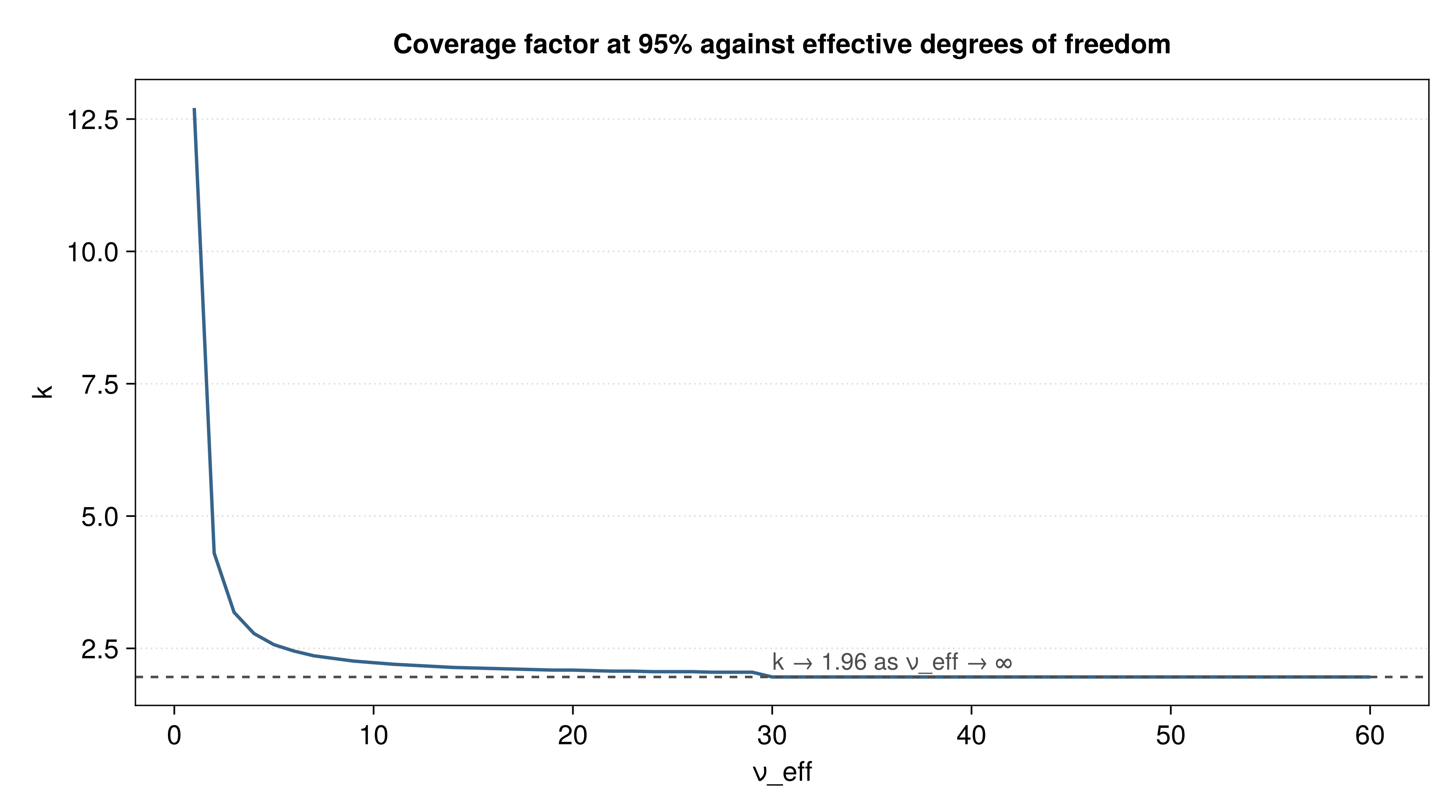
The factor expanded_uncertainty derives at 95% for each number of effective degrees of freedom. It falls steeply: 12.71 at one degree of freedom against 1.96 in the limit, which is what the warning of REQ-175 is about — a short measurement series does not get k = 2.
The small step at ν_eff = 30 is the implementation showing through: below 30 the factor is a Student-t quantile (2.04 at 30), from 30 on it is the normal 1.96. The GUM allows the substitution once ν_eff is large; the figure shows where this package draws that line.
Generated by docs/figures/make_figures.jl from the fixtures in docs/figures/fixtures.jl: computed by the package itself, never copied from a standard (REQ-307, REQ-312).
Welch-Satterthwaite — welch_satterthwaite(contributions, dofs)
See the box at the top of this page — the Welch-Satterthwaite pathway exists precisely to handle the ν_eff < 30 case the k = 2 shortcut cannot.
welch_satterthwaite(contributions, dofs) returns the symbolic effective degrees of freedom per JCGM 100:2008 §G.4 equation (G.2b):
\[\nu_{\text{eff}} = \frac{\left(\sum_i u_i^2\right)^2} {\sum_i \frac{u_i^4}{\nu_i}}\]
@variables u1 u2 ν1 ν2

ν_eff = welch_satterthwaite([u1, u2], [ν1, ν2])
# = (u1² + u2²)² / (u1⁴/ν1 + u2⁴/ν2)
\[ \begin{equation} \frac{\left( \mathtt{u1}^{2} + \mathtt{u2}^{2} \right)^{2}}{\frac{\mathtt{u1}^{4}}{\mathtt{{\nu}1}} + \frac{\mathtt{u2}^{4}}{\mathtt{{\nu}2}}} \end{equation} \]
Mismatched list lengths raise DimensionMismatch. Empty or all-zero inputs return the formal 0/0 symbolic expression unchanged.
End-to-end: from contributions to expanded uncertainty
Combine welch_satterthwaite with the keyword form of expanded_uncertainty to derive the coverage-probability-based expanded uncertainty for a small-sample calibration:
using Symbolics
using SymbolicUncertainties

@variables Vin σVin R1 σR1 R2 σR2
@variables ν_Vin ν_R1 ν_R2

Vout = propagate(
    (vin, r1, r2) -> vin * r2 / (r1 + r2),
    [Vin ± σVin, R1 ± σR1, R2 ± σR2],
)

u_Vin = uncertainty_contribution(Vout, Vin, σVin)
u_R1  = uncertainty_contribution(Vout, R1,  σR1)
u_R2  = uncertainty_contribution(Vout, R2,  σR2)

# Evaluated rather than printed: `Symbolics.substitute` inserts the
# numbers but does not reduce them (see upstream-bugs.md UB-001), so
# the closed form stays enormous. `build_evaluator` is the tool that
# actually produces numbers — see the Code Generation page.
# Volts and ohms; stripped because the evaluation below works on
# plain numbers.
vals = Dict(
    k => ustrip(v) for (k, v) in Dict(
        Vin => 12.0us"V", σVin => 0.1us"V",
        R1 => 1_000.0us"Ω", σR1 => 10.0us"Ω",
        R2 => 2_000.0us"Ω", σR2 => 20.0us"Ω",
    )
)
[
    Float64(eval(Symbolics.toexpr(Symbolics.substitute(u, vals)))) for
    u in (u_Vin, u_R1, u_R2)
]

ν_eff = welch_satterthwaite(
    [u_Vin, u_R1, u_R2],
    [ν_Vin, ν_R1, ν_R2],
)

Vout_with_dof = SymbolicMeasurement(Vout.val, Vout.err, ν_eff)
Vout_U = expanded_uncertainty(
    Vout_with_dof;
    coverage_probability = 0.95,
)
(R2*Vin) / (R1 + R2) ± sqrt((((-R2*Vin) / ((R1 + R2)^2))^2)*(σR1^2) + (((R1*Vin) / (R1^2 + 2R1*R2 + R2^2))^2)*(σR2^2) + ((R2 / (R1 + R2))^2)*(σVin^2))*(1.96 + (2.372384(((abs((-R2*Vin) / ((R1 + R2)^2))^4)*(σR1^4)) / ν_R1 + ((abs(Vin / (R1 + R2) + (-R2*Vin) / ((R1 + R2)^2))^4)*(σR2^4)) / ν_R2 + ((abs(R2 / (R1 + R2))^4)*(σVin^4)) / ν_Vin)) / (((abs((-R2*Vin) / ((R1 + R2)^2))^2)*(σR1^2) + (abs(Vin / (R1 + R2) + (-R2*Vin) / ((R1 + R2)^2))^2)*(σR2^2) + (abs(R2 / (R1 + R2))^2)*(σVin^2))^2) + 2.8227073279999995(((((abs((-R2*Vin) / ((R1 + R2)^2))^4)*(σR1^4)) / ν_R1 + ((abs(Vin / (R1 + R2) + (-R2*Vin) / ((R1 + R2)^2))^4)*(σR2^4)) / ν_R2 + ((abs(R2 / (R1 + R2))^4)*(σVin^4)) / ν_Vin) / (((abs((-R2*Vin) / ((R1 + R2)^2))^2)*(σR1^2) + (abs(Vin / (R1 + R2) + (-R2*Vin) / ((R1 + R2)^2))^2)*(σR2^2) + (abs(R2 / (R1 + R2))^2)*(σVin^2))^2))^2) + 2.5561097948467197(((((abs((-R2*Vin) / ((R1 + R2)^2))^4)*(σR1^4)) / ν_R1 + ((abs(Vin / (R1 + R2) + (-R2*Vin) / ((R1 + R2)^2))^4)*(σR2^4)) / ν_R2 + ((abs(R2 / (R1 + R2))^4)*(σVin^4)) / ν_Vin) / (((abs((-R2*Vin) / ((R1 + R2)^2))^2)*(σR1^2) + (abs(Vin / (R1 + R2) + (-R2*Vin) / ((R1 + R2)^2))^2)*(σR2^2) + (abs(R2 / (R1 + R2))^2)*(σVin^2))^2))^3)) (k = 1.96 + (2.372384(((abs((-R2*Vin) / ((R1 + R2)^2))^4)*(σR1^4)) / ν_R1 + ((abs(Vin / (R1 + R2) + (-R2*Vin) / ((R1 + R2)^2))^4)*(σR2^4)) / ν_R2 + ((abs(R2 / (R1 + R2))^4)*(σVin^4)) / ν_Vin)) / (((abs((-R2*Vin) / ((R1 + R2)^2))^2)*(σR1^2) + (abs(Vin / (R1 + R2) + (-R2*Vin) / ((R1 + R2)^2))^2)*(σR2^2) + (abs(R2 / (R1 + R2))^2)*(σVin^2))^2) + 2.8227073279999995(((((abs((-R2*Vin) / ((R1 + R2)^2))^4)*(σR1^4)) / ν_R1 + ((abs(Vin / (R1 + R2) + (-R2*Vin) / ((R1 + R2)^2))^4)*(σR2^4)) / ν_R2 + ((abs(R2 / (R1 + R2))^4)*(σVin^4)) / ν_Vin) / (((abs((-R2*Vin) / ((R1 + R2)^2))^2)*(σR1^2) + (abs(Vin / (R1 + R2) + (-R2*Vin) / ((R1 + R2)^2))^2)*(σR2^2) + (abs(R2 / (R1 + R2))^2)*(σVin^2))^2))^2) + 2.5561097948467197(((((abs((-R2*Vin) / ((R1 + R2)^2))^4)*(σR1^4)) / ν_R1 + ((abs(Vin / (R1 + R2) + (-R2*Vin) / ((R1 + R2)^2))^4)*(σR2^4)) / ν_R2 + ((abs(R2 / (R1 + R2))^4)*(σVin^4)) / ν_Vin) / (((abs((-R2*Vin) / ((R1 + R2)^2))^2)*(σR1^2) + (abs(Vin / (R1 + R2) + (-R2*Vin) / ((R1 + R2)^2))^2)*(σR2^2) + (abs(R2 / (R1 + R2))^2)*(σVin^2))^2))^3))Because ν_eff here is a purely symbolic expression (not a concrete Real), the keyword form falls back to the normal quantile and emits an @info message. Supply a concrete numeric substitution via Symbolics.substitute to obtain the t-quantile path and the REQ-175 @warn when appropriate.
API reference
U is not a standard uncertainty
expanded_uncertainty returns an ExpandedUncertainty, not a SymbolicMeasurement. This is deliberate.
U = k · u_c is the half-width of a coverage interval. It is a reporting quantity, not an input to further propagation: a value carrying U where u_c is expected inflates every downstream result by the coverage factor, silently and by exactly k. Returning a SymbolicMeasurement would have made that substitution type-correct and therefore easy to make by accident.
The distinct type carries the estimate, U, the coverage factor k that produced it, and the effective degrees of freedom k was derived from — everything a calibration certificate has to state under JCGM 100:2008 §7.2.3, and nothing that invites reuse in a computation.
SymbolicUncertainties.expanded_uncertainty — Function
expanded_uncertainty(m::SymbolicMeasurement, k = 2) -> ExpandedUncertaintyexpanded_uncertainty(m, k) returns U = k·u_c(y) under the GUM §6.3.3 assumption that the output distribution is approximately normal. When the effective degrees of freedom ν_eff < 30, the shortcut k = 2 for 95 % coverage is inadequate; use the keyword form expanded_uncertainty(m; coverage_probability = …) so that k is derived from m.dof via the Student-t quantile of JCGM 100:2008 §G.4.
Return a measurement with val = m.val, err = k·m.err, and dof = m.dof (preserved). The default k = 2 matches EA-4/02 usage and the GUM Annex H worked examples.
Negative numeric k raises ArgumentError. Symbolic k is left in closed form with no sign inspection.
Implements the methodology of JCGM 100:2008 §6.2 equation (18). Traces REQ-050.
expanded_uncertainty(m; coverage_probability=nothing) -> ExpandedUncertaintySingle-argument convenience wrapper. With no keyword argument it applies the default k = 2, matching EA-4/02 usage. With an explicit coverage_probability, it derives k from m.dof via the Student-t quantile of JCGM 100:2008 §G.4 Table G.2.
The keyword form derives k from m.dof via the Student-t quantile of JCGM 100:2008 §G.4 Table G.2. When m.dof is nothing or a symbolic expression, the normal-distribution quantile is used instead (per GUM §6.3.3); a numeric ν_eff < 30 emits a runtime @warn.
Supported coverage_probability values: {0.68, 0.90, 0.95, 0.99} — the four entries of GUM Table G.2. Other values raise ArgumentError.
See expanded_uncertainty(m, k) for the positional form.
Implements the methodology of JCGM 100:2008 §6.2 / §G.4. Traces REQ-050, REQ-051, REQ-174, REQ-175.
SymbolicUncertainties.ExpandedUncertainty — Type
ExpandedUncertaintyResult of an expanded-uncertainty calculation: the estimate val, the expanded uncertainty U = k · u_c, the coverage factor k, and the effective degrees of freedom the factor was derived from.
Deliberately not a SymbolicMeasurement. U is a coverage interval half-width, not a standard uncertainty, so a quantity carrying it is not propagatable: feeding U back into a computation would silently inflate every downstream result by k. Returning a distinct type makes that mistake impossible to make by accident (JCGM 100:2008 §6.2).
Traces REQ-050, REQ-051.
SymbolicUncertainties.welch_satterthwaite — Function
welch_satterthwaite(contributions, dofs) -> NumThe Welch-Satterthwaite effective degrees of freedom support the Student-t pathway of expanded_uncertainty(m; coverage_probability). The k = 2 shortcut of expanded_uncertainty(m, 2) assumes ν_eff ≥ 30; below that threshold, JCGM 100:2008 §6.3.3 requires the t-quantile path this function enables.
Return the symbolic effective degrees of freedom ν_eff per JCGM 100:2008 §G.4 equation (G.2b):
ν_eff = (Σᵢ uᵢ²)² / Σᵢ (uᵢ⁴ / νᵢ)where uᵢ are the per-variable uncertainty contributions (typically from uncertainty_contribution) and νᵢ the associated degrees of freedom.
Raises DimensionMismatch when the two lists differ in length.
Edge case: empty lists or all-zero contributions produce the formal 0/0 symbolic expression unchanged — no special-case substitution to Inf.
Implements the methodology of JCGM 100:2008 §G.4. Traces REQ-052, REQ-174.