Monte Carlo Cross-Validation
The GUM framework linearises the measurement model around the input estimates and reports y ± k·u_c. JCGM 101:2008 propagates the input distributions instead, by sampling, and §8 of that document is explicit about why a GUM user would want it: to validate the framework's result where the linearisation, or the normality it assumes for the output, is in doubt.
monte_carlo runs both and compares them under the §8.2 test.
Loading Distributions alongside this package makes ± ambiguous — it is exported by IntervalSets, which Distributions re-exports — and Julia will resolve neither. A cross-check needs Distributions by construction, so build measurements with the constructor in such a session: SymbolicMeasurement(V, σV) rather than V ± σV. The same trap applies to Measurements.jl; see Interoperability.
You must state each input's distribution
using Symbolics, SymbolicUncertainties
using MonteCarloMeasurements, Distributions

@variables V σV I σI
R = SymbolicMeasurement(V, σV) / SymbolicMeasurement(I, σI)

c = monte_carlo(
    R,
    # Distributions.jl requires dimensionless numbers
    Dict(
        V => Normal(5.0, 0.01),   # V
        I => Normal(0.1, 0.001)   # A
    );
    n = 20_000,
)
Monte Carlo cross-validation (JCGM 101:2008 §8.2)
trials : 20000
GUM y ± u_c : 50.0 ± 0.5099019513592783
MC y ± u_c : 50.00500514270396 ± 0.5104850993513707
coverage probability: 0.95
GUM interval : (49.00061053968912, 50.99938946031088)
MC interval : (49.01799480301342, 51.02740513214836)
tolerance (2 digits) : 0.005000000000000001
NOT VALIDATED — the linearisation is inadequate hereThe distribution of every input is supplied by the caller and is never defaulted. A standard uncertainty is not a distribution: JCGM 101:2008 §6.4 assigns a rectangular density to a Type B evaluation stated as a half-width and a normal one to a Type A evaluation, and the choice changes the answer. Defaulting to normal would also make the exercise circular — a run that assumes normality cannot discover that normality was the wrong assumption.
The first-order side takes each input's estimate and standard uncertainty from the same density, which is what §6.4 means by assigning a PDF to an input quantity: a rectangular half-width a contributes u = a/√3 without the caller restating it.
What the §8.2 test actually asks
It compares coverage intervals, not u_c. Express u_c to ndig significant digits; the tolerance δ is half a unit in the last of them; the framework is validated when both interval endpoints agree to within δ.
That distinction has teeth. Consider an exactly linear model — a sum, which has no higher-order terms at all — with rectangular inputs:
@variables V1 σV1 V2 σV2
S = SymbolicMeasurement(V1, σV1) + SymbolicMeasurement(V2, σV2)

rect = monte_carlo(
    S,
    Dict(
        V1 => Uniform(4.98, 5.02),  # V
        V2 => Uniform(0.096, 0.104) # V
    );
    n = 20_000,
)
Monte Carlo cross-validation (JCGM 101:2008 §8.2)
trials : 20000
GUM y ± u_c : 5.1 ± 0.011775681155103553
MC y ± u_c : 5.1 ± 0.01177343106492013
coverage probability: 0.95
GUM interval : (5.07692008904257, 5.123079910957429)
MC interval : (5.07990439, 5.119970029999999)
tolerance (2 digits) : 0.0005
NOT VALIDATED — the linearisation is inadequate hereThe two u_c agree, and the test still fails: the sum of two uniforms is trapezoidal, so y ± 1.96·u_c is the wrong interval even though the linearisation is perfect. "GUM validated" and "the model is linear" are different statements, and this is the case that separates them.
Conversely the same model with normal inputs passes, because then the output really is normal:
monte_carlo(
    S,
    Dict(
        V1 => Normal(5.0, 0.01),  # V
        V2 => Normal(0.1, 0.002)  # V
    );
    n = 20_000,
)
Monte Carlo cross-validation (JCGM 101:2008 §8.2)
trials : 20000
GUM y ± u_c : 5.1 ± 0.01019803902718557
MC y ± u_c : 5.1 ± 0.010175293395869126
coverage probability: 0.95
GUM interval : (5.080012210793782, 5.119987789206217)
MC interval : (5.079918813216342, 5.120059790835053)
tolerance (2 digits) : 0.0005
VALIDATED — the first-order result agreesFigure — the two intervals side by side
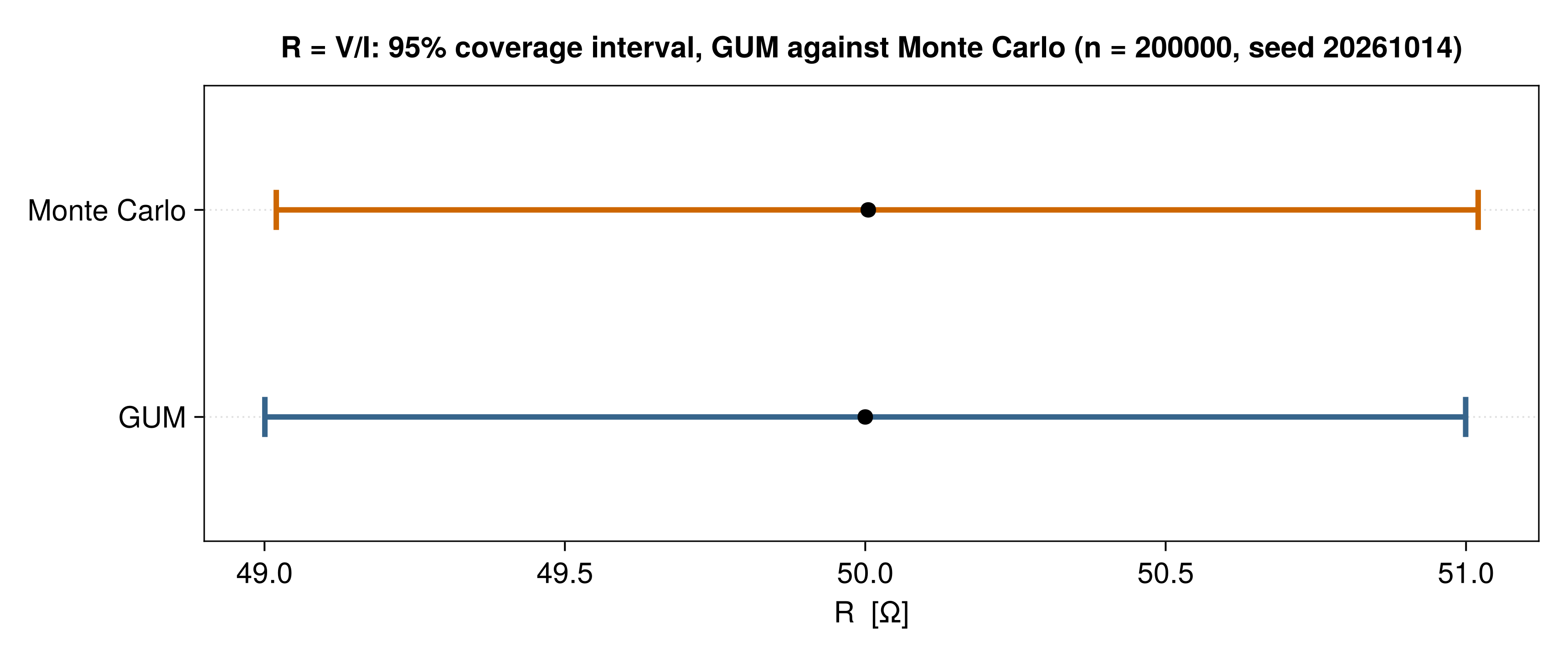
The §8.2 comparison as a picture: the GUM interval and the Monte Carlo interval for R = V/I, with the estimate marked on each. The run is seeded, so the figure is the same on every machine (REQ-309).
Generated by docs/figures/make_figures.jl from the fixtures in docs/figures/fixtures.jl: computed by the package itself, never copied from a standard (REQ-307, REQ-312).
Adequacy is a property of the operating point
Ohm's law at 1 % relative input uncertainty is not validated: a quotient of normals is skewed with heavier tails, so the sampled interval is wider and shifted, by far more than the tolerance — while u_c agrees to four digits. Ten times smaller inputs and the same formula passes. Nothing about the expression changes; the operating point does.
Correlated inputs are sampled jointly
A declared correlation is honoured on both sides. Sampling the inputs independently would silently reproduce the uncorrelated answer, and the comparison would then disagree — or, worse, agree for the wrong reason if the correlation were dropped on both sides too.
a, b = declare_correlated(
    SymbolicMeasurement(V1, σV1),
    SymbolicMeasurement(V2, σV2),
    0.9,
)
d = a - b

monte_carlo(
    d,
    Dict(
        V1 => Normal(10.0, 0.5),  # V
        V2 => Normal(4.0, 0.5)    # V
    );
    n = 20_000,
)
Monte Carlo cross-validation (JCGM 101:2008 §8.2)
trials : 20000
GUM y ± u_c : 6.0 ± 0.22360679774997894
MC y ± u_c : 6.0 ± 0.22404192460027075
coverage probability: 0.95
GUM interval : (5.561738729711709, 6.438261270288291)
MC interval : (5.561576310519559, 6.439706242418839)
tolerance (2 digits) : 0.005000000000000001
VALIDATED — the first-order result agreesThe difference of two strongly correlated inputs has far less uncertainty than the uncorrelated formula would give — 0.5·√(2−2ρ) against 0.5·√2 — and the sampled result must land on the correlated value.
Two refusals guard this path:
- A correlation matrix that is not positive semi-definite has no joint distribution behind it, and is rejected. Pairwise coefficients assigned by hand produce this easily:
ρ(x,y) = ρ(x,z) = 0.9withρ(y,z) = −0.9asks two inputs to track a third closely while opposing each other. - A non-normal marginal on a correlated input is rejected rather than transformed. Correlated sampling here is the multivariate normal of JCGM 101:2008 §6.4.8 — independent standard normals through a Cholesky factor — and that construction preserves the marginals only because they are normal. Imposing it on a rectangular density would quietly replace the density you stated. §6.4.8.4 is where a genuine joint PDF belongs.
A finding: the GUM's own §H.1 does not pass
The end-gauge example of JCGM 100:2008 §H.1 is not validated by the §8.2 test, and the reason is instructive rather than alarming.
Its model contains the product ls·δα·θ, and the Annex estimates δα = 0. The first-order sensitivity to θ is therefore −ls·δα = 0: the framework assigns θ no contribution at all. Sampling multiplies a non-zero δα by a non-zero θ and recovers a variance the linearisation cannot see, of size ls·u(δα)·u(θ) ≈ 12 nm. It appears in quadrature:
u_c (first order) = 31.7 nm
missed term       = 11.9 nm
√(31.7² + 11.9²)  = 33.9 nm   = the sampled value
This is a second-order term in the strict sense — a product of two inputs whose estimates are both zero — and JCGM 100:2008 §5.1.2 note 1 is the caveat it falls under. The package's first-order result is correct: it computes what the GUM prescribes, and reproduces the Annex's published 32 nm. The GUM is the one neglecting the term.
That is the whole argument for this milestone. The Annex H suite checks the implementation against the GUM's own worked answers, and every one of those answers comes from the framework being checked. A cross-check that does not is the only thing that could have surfaced this.
The verdict depends on the number of trials
A tail quantile's standard error falls only as 1/√n, so a verdict computed near the tolerance boundary can flip on a rerun. When the interval discrepancy lands within 25 % of δ, monte_carlo warns: read that as "increase n", not as a property of the measurement model.
adaptive = true removes the guesswork. It is the procedure of JCGM 101:2008 §7.9: draw blocks of n trials until the results have stabilised — twice the standard deviation of the block means, for the estimate, u(y) and both interval endpoints, below the numerical tolerance. Stabilising u(y) alone would miss the point, since §8.2 compares intervals and it is their endpoints that carry the quantile noise.
adaptive = monte_carlo(
    R,
    # Distributions.jl requires dimensionless numbers
    Dict(
        V => Normal(5.0, 0.01),   # V
        I => Normal(0.1, 0.001)   # A
    );
    adaptive = true,
    n = 20_000,
)
(adaptive.blocks, adaptive.converged, adaptive.n)
(10, true, 200000)converged is false for a plain single run because nothing checked it — which is not the same as checked and failed. blocks tells the two apart: one block means no procedure ran. A run that exhausts max_blocks without stabilising warns and reports the block average, flagged as unstabilised.
The procedure is stated for the four scalar results of one measurand. What stabilisation would mean for the correlation matrix of a vector-valued measurand is not something the standard defines, so adaptive = true is refused there rather than guessed at; check each output on its own if you need it.
Several outputs at once
JCGM 102:2011 §6 asks for the covariance matrix of a vector-valued measurand, not only its marginal uncertainties: that matrix is what a downstream user needs to combine the outputs further. Pass a vector, and the inputs are sampled once with every output evaluated on that draw:
Rm = SymbolicMeasurement(V, σV) / SymbolicMeasurement(I, σI)
Xm = Rm * 2.0

res = monte_carlo(
    [Rm, Xm],
    # Distributions.jl requires dimensionless numbers
    Dict(
        V => Normal(5.0, 0.01),   # V
        I => Normal(0.1, 0.001)   # A
    );
    n = 20_000,
)
res.correlation_mc
2×2 Matrix{Float64}:
1.0 1.0
1.0 1.0Two separate calls would not do: they draw independent inputs and measure a correlation of zero by construction — the same defect as sampling correlated inputs independently, seen from the output side.
What it never does
A Monte Carlo run does not alter the symbolic result. It is a check on the framework, not a correction to it — the same posture as linearisation_bound and second_order_correction, which report and never apply.
API reference
SymbolicUncertainties.monte_carlo — Function
monte_carlo(m::SymbolicMeasurement, distributions; kwargs...)Propagate m's measurement model by a Monte Carlo method and compare the result against the first-order one (JCGM 101:2008 §8).
Requires MonteCarloMeasurements.jl to be loaded; the distributions are Distributions.jl objects, one per input variable.
The distribution of each input is supplied by the caller and never defaulted (REQ-231). A standard uncertainty is not a distribution: JCGM 101 §6.4 assigns a rectangular density to a Type B evaluation stated as a half-width and a normal one to a Type A evaluation, and the choice changes the answer. Defaulting to normal would also make the validation circular, since a run that assumes normality cannot detect that normality was the wrong assumption.
Traces REQ-230, REQ-231.
SymbolicUncertainties.MonteCarloComparison — Type
MonteCarloComparisonThe result of cross-checking a first-order GUM propagation against a Monte Carlo propagation of the same measurement model (JCGM 101:2008 §8).
n— total number of Monte Carlo trials.blocks— how many blocks of trials the adaptive procedure of JCGM 101:2008 §7.9 drew;1for a single non-adaptive run.converged— whether that procedure stabilised. It isfalsefor a single run because nothing checked, which is not the same as checked and failed; the two are distinguished byblocks.estimate_gum,u_gum— the first-order estimate and combined standard uncertainty, JCGM 100:2008 §5.1.2.estimate_mc,u_mc— the mean and standard deviation of the sampled output distribution, JCGM 101:2008 §7.6.interval_gum,interval_mc— the coverage intervals compared by the §8.2 validation test, atcoverage_probability.ndig— the number of significant digits ofu_gumregarded as meaningful, which fixes the numerical tolerance of that test.validated— whether the first-order result passes it.
A Monte Carlo run never changes the symbolic result (REQ-234): this is a check on the framework, not a correction to it.
Traces REQ-230, REQ-233.